Introduction

Geophysics observes the behavior of waves propagating within a material. A seismic signal, in fact, changes according to the characteristics of the crossed environment. The waves can be generated artificially through the use of hammers, explosions, etc.

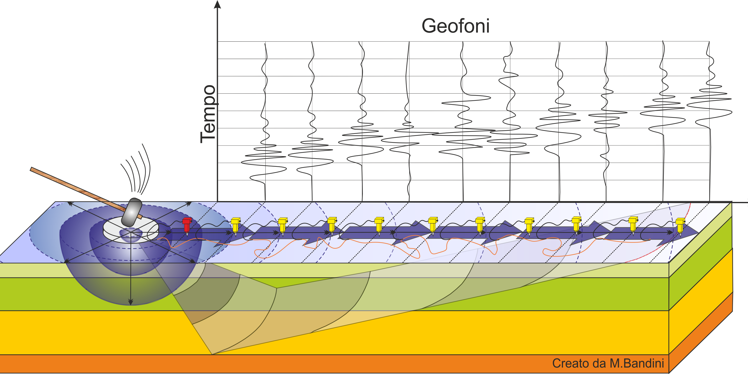
Motion of the seismic signal

The seismic signal can be decomposed into several phases, each of which identifies the movement of particles invested by the seismic waves. The phases are:

• LongitudinalP
• TransversalS
• LoveL
• RayleighR

Rayleigh – “R” waves

In the past, studies on the spread of seismic waves have focused on the propagation of deep waves (P, S) considering surface waves as a disturbance of the seismic signal to analyze. Recent studies have allowed creating advanced mathematical models for the analysis of surface waves in environments with different stiffness.

Signal analysis with MASW technique

According to the fundamental hypothesis of the linear physics (Fourier's Theorem) signals can be represented as the sum of independent signals, called harmonics of the signal. These harmonics, for one-dimensional analysis, are trigonometric functions sine and cosine, and act independently, not interacting with each other. Focusing on each harmonic component, the final result in linear analysis will be equivalent to the sum of partial behaviors corresponding to different harmonics. The Fourier analysis (FFT spectral analysis) is the fundamental tool for the spectral characterization of the signal. The analysis of Rayleigh waves, using MASW technique is performed with the spectral treatment of the signal in the transformed domain, where you can, quite easily, identify the signal for the Rayleigh waves from other types of signals, observing in addition, the Rayleigh waves propagate with a velocity that is in function of the frequency. The velocity frequency link is called dispersion spectrum. The dispersion curve identified in the f-k domain is called the experimental dispersion curve, and in that domain represents the maximum amplitudes of the spectrum.

Modelling

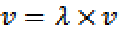
From a synthetic geotechnical model characterized by thickness, density, Poisson's ratio, S and P wave velocity it is possible to simulate the theoretical dispersion curve, which links velocity and wavelength according to the correlation:

By changing the parameters of the synthetic geotechnical model, it can be obtained an overlay of the theoretical dispersion curve with the experimental one: this is called inversion and is used to determine the profile of velocities in environments with different stiffness.

Vibration modes

Both in the theoretical and experimental inversion curve it is possible to identify the different configurations of vibration of the ground. The modes for the Rayleigh waves can be: deformation in contact with the air, almost no deformation of the half-wavelength and zero deformation at high depths.

Depth of investigation

The Rayleigh waves decay at a depth approximately equal to the wavelength. Small wavelengths (high frequencies) are used to investigate superficial areas and large wavelengths (low frequencies) allow investigations to a greater depth.

The workflow in Easy MASW: from the recorded data to the Vs profile

The goal of a MASW survey is to obtain the profile of the shear-wave velocity Vs as a function of depth, starting from the vibrations recorded at the surface by the geophones. In Easy MASW the path is always the same and consists of four steps:

1. Trace import. The seismograms recorded by the geophones during the spread are loaded: they are the raw starting data.

2. Spectral analysis. The software transforms the traces into a dispersion image: a coloured map whose horizontal axis is the frequency and whose vertical axis is the phase velocity. The brighter, higher-energy zones draw "ridges": each ridge is the dispersion curve of one vibration mode of the ground (fundamental mode and higher modes).

3. Picking. The coloured ridges are turned into numerical points. By clicking along a ridge you extract, mode by mode, the experimental dispersion curve: this is the measured data on which the whole subsequent computation is based.

4. Inversion. The Vs profile that reproduces the picked curve is searched for. The result is the velocity stratigraphy (thickness and Vs of each layer), from which the equivalent Vs and the soil category are then derived.

The principle in one sentence

Surface waves are dispersive: low frequencies (long waves) penetrate deep and "see" the deep layers, while high frequencies (short waves) stay near the surface. This is why the phase-velocity/frequency curve carries the information about the Vs profile of the subsoil. Measuring it (picking) and working back to the profile that generates it (inversion) is, essentially, the whole MASW method.

You do not need to know the stratigraphy beforehand

The ground stratigraphy is not a datum you enter at the start: it is the result you obtain at the end, with the inversion. Everything you set before — the optional synthetic model in the spectral analysis and the search limits in the inversion — only guides the computation, it is not the solution.

In short, the workflow is:

Geophone traces
   →  Spectral analysis   (frequency–velocity map: the ridges are the modes)
   →  Picking             (extract the experimental dispersion curve, one per mode)
   →  Inversion           (find the Vs profile that reproduces the picked points)
   →  Vs profile · equivalent Vs · Soil category   (the result)

© Geostru