Understanding seismic refraction
This page explains what a seismic refraction survey measures and why it works. If this is the first time you have dealt with this type of survey, read it before using the software: almost every choice EasyRefract asks you to make (how many layers, where the first arrival falls, which velocity to choose) becomes obvious once the principle is clear.
1. What it is
Seismic refraction is an indirect geophysical prospecting method: it does not excavate and it does not take samples. A seismic pulse is generated at the surface and the time the wave takes to reach a series of receivers (geophones) laid out in line on the ground is measured. From the arrival times the wave velocity in the various materials is derived, and hence the geometry of the subsoil.
The waves generated are of two types: P waves (primary, compressional) and S waves (secondary, shear). Refraction works on P waves, because they are the fastest and therefore the first to be recorded: it is their arrival instant — the first arrival — that is the only datum you will have to read on the seismograms.
2. Why the wave "comes back up": total refraction
When a seismic ray meets the surface separating two materials with different velocities (\(V_1\) above, \(V_2\) below), it is refracted according to Snell's law. The angle changes depending on the ratio between the velocities:
- if \(V_2 < V_1\) the ray becomes more vertical and is lost at depth: it does not come back to the geophones;
- if \(V_2 > V_1\) the ray tends instead to become more horizontal.
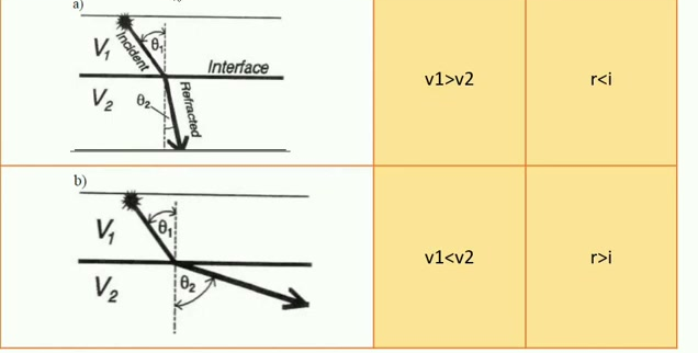
The two cases. In a) velocity decreases downwards (\(V_1>V_2\)): the refracted ray bends away from the interface and is lost at depth. In b) velocity increases (\(V_1<V_2\)): the ray bends towards the horizontal, and this is the only case useful for the survey.
As the angle of incidence increases, a particular value is reached — the critical angle — for which the refraction angle becomes exactly 90°: the ray travels along the discontinuity surface, at the velocity \(V_2\) of the lower layer. This is total refraction.
While it runs along the discontinuity, the ray behaves like a continuous wave generator: it releases energy upwards, returning a family of rays parallel to one another and inclined at the critical angle. These are the head waves (or conical waves), and they are what the geophones record.
The fundamental condition
Total refraction occurs only if velocity increases with depth (\(V_1 < V_2 < V_3 \dots\)). If a deeper level is slower than the one above it, the method does not see it: this is not a software or instrumentation problem, it is a physical limitation of the method.
3. Direct wave and refracted wave: the crossover point
Two families of waves reach the geophones:
- the direct wave, which travels at the surface at the velocity \(V_1\) of the shallowest layer, along the shortest path;
- the refracted wave (head wave), which follows a longer path — it goes down, runs along the refractor, comes back up — but covers a stretch at the higher velocity \(V_2\).
At the geophones close to the source the direct wave arrives first, because the path is short. But as you move away, the fast stretch at \(V_2\) becomes longer and longer and at a certain point the refracted wave catches up and overtakes the direct one: the point at which the two are equivalent is the crossover point. From there on, the first arrival you read is no longer the direct wave, but the refracted one.
4. The traveltime curve: the diagram we will use
By plotting the geophone distance (X axis) against the first arrival time (Y axis) you obtain the traveltime curve (or time–distance curve).
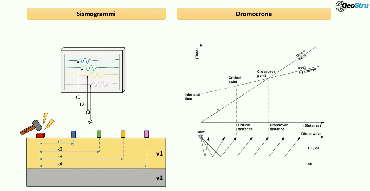
Left: each geophone, at distance \(x_1 \dots x_4\) from the source, records a seismogram from which the first arrival time \(t_1 \dots t_4\) is read. Right: those same times plotted against distance form the traveltime curve. The direct wave, the first head wave and the crossover point — where the latter overtakes the former — can be recognised.
It is the heart of the interpretation, because:
- each straight segment corresponds to a wave travelling in a material at constant velocity;
- the slope of that segment is the inverse of the velocity: the flatter the segment, the faster the material;
- the knee points (the slope changes) are the crossover points, that is the transition from one wave to the next.
Hence the rule you will use continually in EasyRefract:
Layers and refractors
A refractor is the surface separating two layers. Therefore: N layers ⇒ N−1 refractors. If on the traveltime curve you recognise the direct wave plus two refracted segments, you have 2 refractors and therefore 3 layers. Counting the slope changes is the practical way to decide how many layers to set in the software.
5. How data are acquired in the field
The spread is the line of geophones. The source — sledgehammer, seismic gun or explosive charge — is fired at different positions, called shots. The source–geophone distance is called offset.
The classic layout, the one also used in the tutorial example, provides for 5 shots:
| Shot | Position | Name |
|---|---|---|
| 1 | outside the spread, before the first geophone | external direct shot |
| 2 | at the head of the spread | direct shot |
| 3 | at the centre of the spread | central shot |
| 4 | at the tail of the spread | reverse shot |
| 5 | outside the spread, after the last geophone | external reverse shot |
Both direct and reverse shots are needed because a dipping refractor gives different times depending on the direction in which it is "crossed": only by combining the two directions can the true refractor velocity be separated from the effect of the dip.
6. What the G.R.M. method does
EasyRefract interprets the data with Palmer's (1980) Generalized Reciprocal Method (G.R.M.). The earlier methods (reciprocal shooting, delay time, plus–minus) worked well only with refractors of gentle and regular dip.
Palmer introduces the optimum XY parameter, which makes it possible to reconstruct even irregular surfaces or surfaces with abrupt variations. The geometrical idea: the projection of each geophone onto the discontinuity is treated as the radius of a circle; by drawing these arcs beneath all the geophones, the refractor is the envelope of tangents to the circular arcs.
An important practical consequence follows: the closer the geophone spacing, the more detailed the refractor and the more reliable the interpretation.
7. Limitations to know before you start
When refraction gets it wrong (and does not tell you)
- Velocity inversion — if a deep layer is slower, the method fails: that layer is not detected.
- Hidden layer — a layer with a velocity intermediate between the one above and the one below may be "skipped over" and not appear.
- Thicknesses that are too small — a layer that is too thin does not produce a recognisable segment on the traveltime curve.
- Geophone spacing — widening it increases the investigated depth but worsens the accuracy of the depths.
- Non-uniqueness — the same times can be explained by more than one model. Where possible, calibrate the interpretation against a borehole.
One last warning that will come in useful at the end, when you assign a lithological name to the layers: velocity does not by itself identify a lithology. Within the same material velocity changes with compaction, fracturing and porosity.
Now that the principle is clear, we can move on to practice: continue with Initial data.