How to import the data
Objective of this step: to bring the seismograms recorded by the seismograph into the software and to tell the program where the geophones were. One shot = one file = one column in the software. In the example we will import 5 shots, following the layout described in Understanding seismic refraction.
Importing the first shot
- Click on Data input, in the vertical bar on the left.
- Move to the folder-shaped icon (Import traces).
- Select the correct format and load the file: in the example an Ambrogeo
file
*.dta. The standard SEG-2, SEG-Y, SU and ASCII formats are also supported.

Declaring the geophone positions
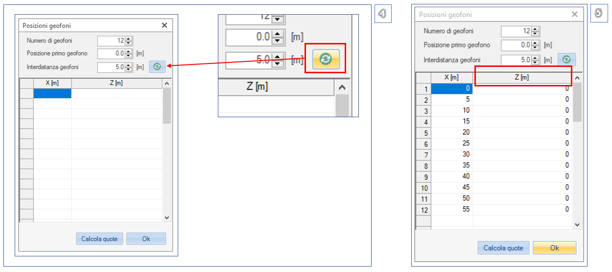
Once the first trace has been loaded, the Geophone positions window appears. Click on update (the circular arrows) and fill in:
- number of geophones (12 in the example);
- position of the first geophone (6 m in the example);
- spacing between the geophones (3 m in the example).
If the geophones are not all at the same elevation, assign the elevation Z [m] of each one: the default value is 0, but on sloping ground it must be corrected, otherwise the calculated depths will be referred to a ground surface that does not exist. You can go back and edit them at any time from Project → Geophone positions. When you have finished, press ok.
They must match the actual spread
Number, position and spacing must reproduce exactly the geometry laid out in the field. It is the easiest mistake to make and it propagates through the whole processing: the distances are the X axis of every traveltime curve.
Adding the subsequent shots
- Press the «+» button (Add shot): a new column appears.
- Import the trace of the new shot with the procedure described above.
- Repeat until all the shots have been loaded.
If you have loaded a file by mistake, remove it with the «−» button (Remove shot).

Now you have to tell the software where each shot was fired from: Shot points, data filtering and first arrivals.